Jusletter IT

The term «collegiate body» refers to an organizational structure within which the decision-making power is shared between two or more persons. These bodies are also known as collegiate chambers, councils or committees.

Influencing factors of the decision-making process have been the focus of various studies conducted by several experts from diverse areas such as jurisprudence or political science. In the legal area, Schubert raises the following question: «To what extent are public acts of judges influenced by their personal beliefs?»¹. The use of theoretical statistics or computer models allows for a better insight in the decision-making process of the members of the collegiate body. Based on this, different studies about decision-making were collected in order to verify the variable types that can be used and the different methods available.

One of the advantages of model creation is the possibility to describe a large quantity of relations with a certain degree of precision, besides being relevant in multidisciplinary research².

Among the existing decision making models, it is necessary to include new characteristics to verify if they can contribute to the vote’s projection or present a larger influence than other variables on the projection. The addition of variables like «intentions», which are not allowed by statistic models, allows working in a dynamic way.

The main problem identified is the inherent complexity in quantifying personal characteristics and the vote’s projection of the collegiate members, due to the large number of existing variables that can influence the votes. It is also difficult to find a generic model adaptable to the various issues addressed by the collegiate body, because each country and topic of the trial agenda has their peculiarities. Moreover, the application of statistic models to the vote’s projection cannot represent appropriately the dynamics present in the processes.

Given the problem above, this study had as objective to test new variables to verify if they contribute to the decision-making model, based on models and variables used in other countries³. Moreover, it verified the model behavior and the results of specific scenarios and interaction variables.

The following will discuss some issues related to statistics, in order to clarify some terms used in the analysis of the data and to understand the model. The model suggested in this study used a regression and a classification model. Despite their differences, both contributed to the selection of the most important variables.

According to Han⁴, classification is the process used to find a model or function, which describes and distinguishes data classes to enable the utilization of the model to predict the objects classes whose value is unknown. The classification models are generally used to predict categorical variables.

Among the several existing classification methods, the decision tree was chosen in order to be suitable for the study proposal, as well as appropriate for exploratory knowledge discovery from the data⁵.

A decision tree can be defined as a flowchart with tree structure in which each node represents tests of an attribute value or attribute values and each branch represents a test result. As for the leaves, they represent classes or class distributions.

It is necessary to identify some procedures to get to the decision tree model. The first step is to select a sample of the data and to separate it in tuples, of which the class is known, to apply a predefined classification algorithm and to obtain a model that represents the sample data.

The second step consists of obtaining the accuracy of the model and the classification of the new data. It is necessary to define a new sample, the test sample to test the accuracy, because the model tends to be highly adjusted to the training data (overfitting).

After the application of the classification rules on the test data (whose class is also known), it is possible to get the accuracy of the model, which is a percentage of tuples (data) that were classified correctly.

If the value of the accuracy is satisfactory for the case study proposed, the classification rules can be applied on data with unknown classes and thus establish projection values.

Regression is a statistical method used to explore and infer relations between variables. According to Levine et al.⁶ the variable to be predicted in a regression is called dependent and the variables used to make the prediction are called independent variables.

Among the various existing regressions are the simple linear, multiple linear and nonlinear. This paper will address the binary logistic regression model, a nonlinear model that is specifically designed for binary dependent variables, as discussed in this article by the variable vote.

Stock and Watson⁷ state that a regression with a binary dependent variable Y models the probability that a given value of dependent variable occurs, so it adopts a nonlinear formulation which does not oblige the predicted values to stay between zero and one, being used in the probit and logit regressions. The probit regression uses the cumulative distribution function (c.d.f.) normal pattern. Logit regression already uses the c. d. f. logistics.

The logit model of the population, from the binary dependent variable Y with multiple regressors X = (X₁, X₂, ..., X_k) is calculated as follows:

where:

β₀ = model constant;

β₁, ..., β_k = coefficients of each predictor variable.

The coefficients of the logit model can be estimated by maximum likelihood. Stock and Watson also mention that the estimator is consistent and normally distributed in large samples such that the statistical t and the confidence intervals for the coefficients can be constructed in the usual way.

Different existing models, both theoretical, as examples of applications with data from other countries courts, will be covered in the following chapter.

According to Hwong⁸, there are five ways to explain judicial decision-making: through legal models, attitudinal, personal, strategic and institutional attributes. It is noteworthy that these models can be used together, to identify the behavior of a court.

However, the models mentioned above are legal, in other words, they only provide theoretical basis for the choice of variables. Therefore, statistical models contribute to the implementation of the model suggested in this article.

Hwong's study explored the influence of socio-demographic characteristics (political and regional ties, sexual gender, and years of experience as a lawyer, among others) of the judges in their decisions on tax law. The study contributes three ideas to the understanding of the legal decision making of tax law. The first idea is that socio-demographic characteristics are influenced variables, namely judges with similar characteristics tend to have the same behavior during the trials. The second idea is that each court has its set of socio-demographic variables and their value of influence. The third is that a quantitative analysis helps to better understand how legal decisions are made, aggregated to a subsequent qualitative analysis.

Although the analysis explores the behavior of judges, it does not explore their individual, but rather their collective behavior in a collegiate body. Hwong used two models as a base, the personal attributes model and the Schneider model, together with Bivariate and Multivariate analysis.

Martin et al.⁹ study in the area of statistic models of decision-making tries to predict results of processes not yet judged by the US Supreme Court. After the real decision of the cases, they compare the outcome with the expected results. For this, Martin selected cases that were pending in the US Supreme Court and applied two different methods to compare the results.

The first method consists of applying a statistical model based on information derived from past decisions of the Supreme Court prior to the case being predicted, in which classification trees were constructed based on the characteristics of each case. The second method, a quantitative analysis, is based on judgments of experts and researchers in the legal field that can have opinions based on the laws, books, and opinions of courts, political and ideological preferences.

After analyzing 628 cases previously decided, Martin created classification trees, which are quoted for them as statistical model. Six characteristics were obtained for each case to be used as explanatory variables, as follows: (a) The court origin of the case, (b) Case theme, (c) Type of process author (e.g. USA, harmed person, company, others), (d) Ideology of first instance decision and (f) Process author argued on the constitutionality of a law.

Cameron and Cummings created a model using concepts of social economy and effects of neighbors or peers (neighborhood/peer effect), such as committing crimes, drinking alcohol, teenage pregnancy, smoking among adolescents, school dropout and others.

In the study of Cameron and Cummings¹⁰ some very important values for the model are mentioned, such as usefulness to the judge of each type of pronounced vote ν_i, where  that uses as a basis the characteristics of a judge i itself, the impact of the characteristics of other voting judges in i judge and the impact of the votes of the other judges in the vote of the judge i. The h_i(ν_i) value represents the utility of the vote of the judge i for himself; θ₁ represents an adjustment coefficient to define the influence of the judges vote in the voting judge; , the usefulness of the i judge vote for the group; is the average value of the votes of the other judges who are judging and ε_i (ν_i) is the peculiar behavior of the judge i.

The private utility reflects the value of the judge i vote, in what he believed to be correct, based on the information he has on the case, understanding of the law, case law (collected body of decisions written by courts) and personal convictions, in addition to the possible influence of other collegiate judges. The social function utility (S_i) is calculated by the following formula  where in the case of three judges, if the judges 2 and 3 vote the same way, the judge 1 receives the value 1 for social utility; if he votes the same way, otherwise he will receive 0. But if the judge 2 votes one way and the judge 3 other way, the judge 1 will receive 0.5, regardless of his vote.

This section presents the research methods steps for the development of the model proposed in this article.

The first task is the development of the document data extraction prototype, together with the definition of the data source that provides documents publicly on their websites.

It is necessary to choose a type of subject matter and a collegiate chamber to analyze data and monitor the collegiate members’ behavior in accordance with the subject, since it can vary depending on the published subject. The criterion for choosing the court was to make documents available in HTML (Hypertext Markup Language) to allow its extraction viably. Thus, the Superior Court of Justice, a Brazilian judiciary court that judges collegially part of the cases, was chosen.

The subject matter chosen was «Tax». The criteria for choice took into account its relevance, its considerable amount available in the chosen court and being an ongoing issue in time.

The second task is to determine which data is available in these documents to recover the information and enter them into a database.

The third task is to verify the integrity of the extracted information. To do so a sample of the data must be selected using the simple sampling technique for manual verification of the documents, to see if the data are consistent with what has been entered in the database

With the data, the value of the judges’ ideology is calculated. The ideology value can be calculated according to the votes of collegiate members extracted from the documents. The W-NOMINATE algorithm from Keith Poole and Howard Rosenthal was used to calculate this value¹¹.

Two different models were selected for the creation of the models, the logistic regression model and the decision tree. The binary logistic regression model was chosen because it does not require the independent variables to have a normal distribution or similar variance. Furthermore, this model assumes that the independent variables should have a linear relationship with the dependent variable, and it is generally used when there are many non-linear effects between the variables, i.e. viable for social science data that show this behavior. But the decision tree was chosen by the fact that it is a simple model, easy to apply and capable to identify the most important variables to project the dependent variable.

The use of Cameron and Cummings model for the section of attributes and for the development of the models was attempted.

As for the selection of variables that will compose the models, all variables available in the curricula of the collegiate members and documents have been identified.

Next a bivariate correlation of all variables was carried out to verify if they attend the rule of not having a high correlation that harmed the regression.

Initially, all variables are used in order to identify which have more influence than others. However, it is possible to redefine the number of variables in a more refined model for the study case.

The evaluation of the logistic regression model is different from the decision tree model; each one has parameters that must be assessed.

In the binary logistic regression model, one should check the overall model and the variables. One should verify the following values to evaluate the overall model: initial verisimilitude Log, which represents the model of adhesion value when no predictor variable is included, and the log verisimilitude end, which is the model of adherence value when all predictors’ variables are included. In addition there is the R² value of Cox and Snell¹² and R² Nagelkerke¹³ which are metrics for evaluating the quality of the model and vary between 0 and 1.

The R² values can range from 0 (forecasters are useless in predicting the outcome variable) to 1 (the model predicts perfectly the output variable). For example, if the R² value of the model is 0.8234, which means that 82.34% of the dependent value can be explained by the present regressors. However, it is common to find the low R² value in social sciences phenomena, as quoted by Hosmer and Lemeshow¹⁴.

As for the evaluation of variables in the model one should pay attention to the following values (a) B: Variable value that is used in the logistic regression equation to design the dependent variable; (b) Standard Error associated with the constant value; (c) Wald: used to evaluate if the statistical parameters are significant. The greater than zero is for the predictor, the more it contributes to the prediction of the output variable; (d) Sig: it is conventionally defined that if the value is <0.05 indicates that the variable is significant in the model. It must be analyzed together with the value of Wald; and (e) Exp (B): Exponentiation of the coefficient B. If the value is greater than 1, the extent to which this value increases, increase the chances of experiencing a given output. If it is less than 1, as the predictor increases, so the chances of determinate output to occur decreases¹⁵.

Note that the selection of variables that best represent the model, impacts on the values which represent the general model quality. In the decision tree model one can evaluate the general model using the following values: the number of instances classified correctly and incorrectly, and Kappa statistic, which is the agreement measure used in nominal scales.

For the simulation the transparency of the simulation behavior and the effectiveness in the presentation of its results were considered. According to Lorscheid¹⁶, this process can be divided into several stages: 1) conception of the model, 2) model construction, 3) check, 4) validation and 5) sensibility analysis.

In the simulation the NetLogo environment was used. The NetLogo is a multi-agent programmable modeling environment used to simulate natural and social phenomena.

The application of NetLogo in this article allows the possibility of the creation of agents representing the members of a collegiate and guide their behavior according to the created models (decision tree and binary logistic regression), and the insertion of new interaction variables. From the application of the models one can test numerous scenarios and agents behavior according to the defined characteristics.

After collecting the data and the proper classification of attributes, the data were applied to regression and decision tree models in order to obtain the coefficients for the equation and the rules of the decision tree, respectively. With the results it was possible to refine the model in order to reduce its complexity with the selection of the attributes that most influence the response variable.

The first task for the decision making model development applied to the legal domain is the analysis of the attributes that the rulings/collegiate members have and what the studied models feature.

After analyzing the data documents and collegiate member and the research variables suggestions available online¹⁷, the following variables accompanied by their type were identified: (a) year of birth (discrete); (b) process rapporteur (dichotomous); (c) status of the member (nominal); (d) sexual gender (dichotomous); (e) educational level (ordinal); (f) ideology (continuous); (g) race (dichotomous); (h) type of university study (dichotomous); (i) university study; (j) status of the process; (k) type of defendant (nominal); (l) type of author (nominal); (m) the rapporteur’s vote; (n) collegiate (nominal); (o) president of Brazil (nominal); (p) year of birth indicator; (q) schooling indicator; (r) race indicator; (s) type of university study indicator; (t) sexual gender indicator and (u) ideology indicator.

The calculation of variables which name contains the word «indicator» used the simple average of the colleagues attributes. However, for future works, one can use another type of calculation. This analysis is important to understand the context in which the variables are located.

It is worth mentioning the attributes used in the Cameron and Cummings model and that could be identified in Brazilian case law: (a) ideology; (b) sexual gender; (c) year of birth; (d) sexual gender indicator; (e) ideology indicator; (f) year of birth indicator; (g) race; (h) race indicator; (i) status of the process, in which the last is equivalent to the court origin, mentioned in the study of Cameron and Cummings. These attributes are important because they are used in the suggested model comparison.

The multiple regression was used to project votes (positive or negative). As the dependent variable, all the other attributes (process characteristics, colleagues and collegiate member) were used.

Before performing logistic regression and getting the model, special treatment should be given to the categorical variables, which is called categories encoding of the qualitative variable.

When the variables are dichotomous to estimate the models parameters, these variables should be replaced by numerical values. However, when the categorical variable has more than two categories, it is necessary to encode them to allow insertion of the values by category in the regression equation.

After converting the categorical variables, the coefficients were calculated to provide the maximum verisimilitude, obtaining the equation that allows determining the probability of a vote to occur.

The coefficients demonstrate the effect of each independent variable with respect to the dependent variable.

The equation below used the logistic regression method with the variables coefficients to estimate the probability of a positive vote to occur, with the cut off value (0.5> 0.5 positive vote and <0.5 negative vote).

Thus, if P (1)> 0.5 the probability of positive vote occurence is greater than the probability of the negative vote, and it can be inferred that the vote is positive in this case.

To evaluate the model, one should verify the data of the coefficients and insert them in the regression model and use them in the testing sample. The sample training, used to run the regression, represents the data selected through stratified sampling technique to model training, which is composed of 2/3 of the total number of positive vote’s records and 2/3 of the total number of negative vote’s records. The testing sample is a sample that was used to validate the model (1/3 of the total data for each type of voting).

After running the regression with all variables, a similar percentage of correct answers for the training sample (65.7%) and testing sample (65.4%) and a low prediction for the positive votes (31.93% for training sample and 31.94% for testing sample) were obtained.

The variables identified as significant in the regression model were the Collegiate, type of defendant and President of Brazil.

The J48 algorithm was applied to the decision tree model with the variables mentioned above. Subsequently, the algorithm was applied using only the variables identified as relevant in the regression model to see if there was a gain on the vote projection.

Before applying the J48 algorithm some parameters were set for the algorithm execution, as the confidence factor and the minimum number of instances per node. The confidence factor is used to perform pruning, where lower values mean larger pruning, the value used in this case was 0.25, default value of Weka Program and also the value by which a higher percentage was obtained correctly. The minimum instances number per leaf was set as 2, default value of the Weka program. However, if the data have too much noise it is necessary to increase this value.

As a result of the application of J48 using all variables a similar percentage of correct answers for the training sample (86.12%) and testing sample (81.33%) and favorable forecast for the positive and negative votes, with error of only 12.71% and 29.94% in the testing sample respectively were obtained. Despite the fact that the decision tree model presents a better result compared to the regression model, the tree model does not quantify the influence of each variable.

The agent’s behavior in the simulation created in NetLogo takes place as illustrated in Figure 1. The simulation in this environment makes it possible fo the user to test various scenarios through a control screen. However, the user can also simulate and observe, using interaction variables, how much they influence the final result of each vote.

The first interaction variable is the probability of a collegiate member to change his vote to follow a colleague, that is, after calculating the one’s vote according to a model (decision tree or regression), this may change one’s vote. The second interaction variable is related to the first, by the fact that it is likely to change the vote. One can follow the vote of a random colleague, or, follow the vote of one member who has been followed more by others vote’s throughout his career, it may be inferred that it has a greater influence.

The user has a screen that can control the simulation variables (features processes and members who are deciding), and visualize the graphs obtained by simulation values.

The simulation aims to examine the influence phenomenon of various attributes in the collegiate member’s votes. The analysis of the characteristics with the greatest influence are important to test scenarios and possible outcomes of the simulation created from the NetLogo environment.

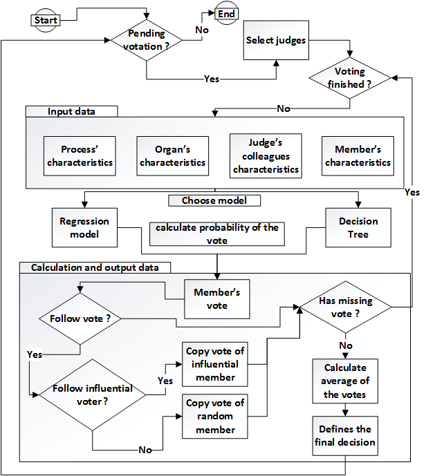
Figure 1. Flowchart of the simulation behavior.

The variables are classified in two steps to display the simulation. First, the simulation parameters are used as reference points to identify all model variables. The parameters that influence model behavior and the parameters used to evaluate the model are included as variables. The «support parameters» are used to calculate the simulation results, as the individual votes and the final voting process (average of the votes).

The variables were classified as independent, dependent or control variables to get an overview of the model components. The dependent variables are the vote and the probability associated with it. The independent variable is the method which will estimate the votes, and the control variables are those which are possible to manipulate to verify the projected vote.

After defining the variables, a simulation which involved creating processes with features according to the values defined in the control variables from the simulation screen was created.

It is noteworthy that two interaction variables were inserted in the simulation: 1) the probability of a collegiate member to follow another voting member and if it happens, it will be applied to 2) the likelihood to follow the most influential voting member. The influence in this case is calculated by the number of times that a member has its vote followed, whose value can be increased during the interactions.

In order to check the impact of the interaction variables in the amount of positive and negative votes obtained during the simulation, an algorithm was developed in NetLogo environment. The table 1 values were used for the experiment among the several existent parameters of the simulation.

The «total members process» values were chosen because they are the same ones used in Tanford and Penrod study¹⁸. The «judge days number» were randomly chosen and can have a big impact on the result, because in each rerun of the algorithm the vote can be changed if the change of voting probability value is greater than 0.

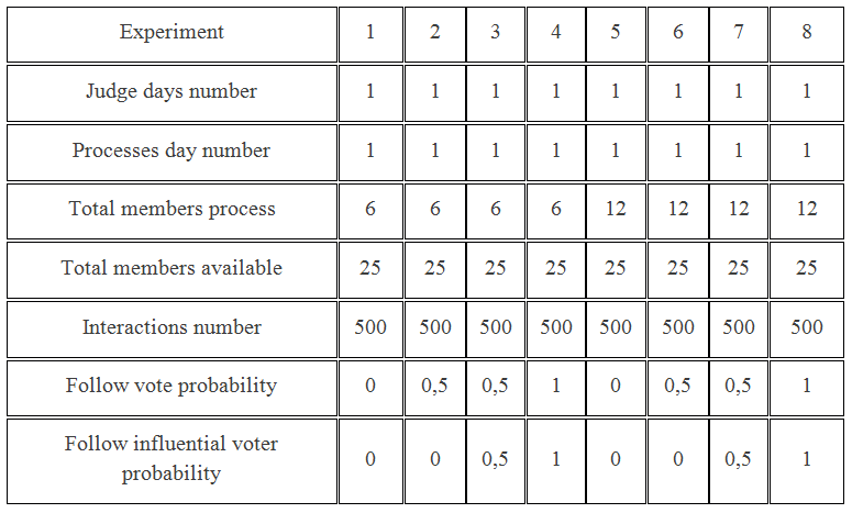
Table 1 Values of input parameters in NetLogo environment.

The «process day number» variable has no direct impact on the votes, only implies the number of process that will be created by the algorithm re-execution. The «total members available» variable represents the number of members that a court has and are available to participate in the voting (polls). Furthermore, for each process the members are randomly selected.

The «interactions number» variable represents the amount of re-execution of the algorithm already executed and the «follow vote probability» variable, the first interaction variable of the system, is the probability that a collegiate member changes its vote.

The second interaction variable, the «proceed influential probability» depends on the «follow vote probability», because only if the «follow vote probability» is greater than 0, the «proceed influential probability» is applied, and if it is 0, a random member shall be selected instead of an influential.

The choice of regression model was made because it contains the coefficients that indicate the influence level of each variable in the vote projection.

The data on Table 2 shows the simulation results, representing the amount of positive votes by coalition for each experiment (e.g. On line 3, experiments 1 through 4 shows 36, 50, 47 and 0 occurrences respectively for the amount of 4 positive and 2 negative out of 6 votes by coalition). It shows that with larger collegiates there are less occurrences of coalitions in which the majority of votes are positive.

Table 2. Results obtained with experiments (1 – 8) in NetLogo environment by type of voting coalition.

The impact of the vote’s amendments in the final outcome of the processes can be seen in Figure 2, which shows the impact of the variables interactions in the final outcome of the proceedings when there was a change of votes.

Figure 2. Graph of the conducted experiments.

One can still check the amount of processes with positive and negative outcome. Subtitles «positive influence» and «negative influence» indicate the end result when there are changes of the member’s votes. The lines of positive and negative votes represent the original vote. When changed by the influence of other members, it was kept in as auxiliary variable to facilitate the comparison.

Given the study above, it is concluded that the simulation and the suggested models, including logistic regression and decision tree allow to project individual votes of a court’s members during a trial. The data used par projection only identifies the probability of a vote to occur according to the data used for model training.

The main contribution of this article is to model the scenario of a collegiate body and how the members behave according to the influence variables. Thus, new variables that can influence the vote’s projection in groups were suggested.

It was possible to compare the result of the vote’s projection with the suggested models and a more refined statistical analysis allowed the reduction of the variables amount used for obtaining a similar result to the full model using all predictor variables. In the full regression model 65.4% of overall accuracy with 21 predictor variables was obtained and the adjusted regression model obtained 61.1% with only three variables.

It was obtained a low predictability of positive votes using the variables mentioned in the Cameron and Cummings model. This fact shows that their model did not work well with the brazilian judicial data.

In addition to the value obtained in the regression by the ideology calculation performed with the Poole et al. algorithm¹⁹ and the voting data, it was possible to obtain a higher amount of success; however, the algorithm does not consider the process characteristics and the parties during the voting process, which this study focused on.

Although it is possible to simulate trials, the model did not meet some statistical parameters, such as high R² from the selection of some attributes available online about the collegiate members and documents. However, according to Wooldridge²⁰, it is common to find lower values for R² in the social sciences, such as between 0.1 and 0.3, but it does not imply that models with these values must be unused.

As future work, the search for new variables is indicated to add them to models and to see if they have a considerable effect in addition to individualized analysis and in existing variable groups. The search for new variables can become a difficult task, since there is no information available ready for use, like the activities carried out by members throughout their professional career.

Aline Macohin. Attorney at Law; Systems Analyst; Phd Candidate in Law at the Federal University of Paraná-Brazil.

Cesar Antonio Serbena. Associate Professor of Legal Philosophy at the Federal University of Paraná-Brazil.

Cameron, C. M. and Cummings, C. P. 2003. Diversity and Judicial Decision-Making: Evidence from Affirmative Action Cases in the Federal Courts of Appeals, 1971-1999.

Cox, D. R. and Snell, E. J. 1968. A General Definition of Residuals. In: Journal of the Royal Statistical Society. Series B (Methodological). Wiley, v. 30, n. 2, p. 248-275.

Field, A. 2005. Discovering Statistics Using SPSS. Sage Publications.

Han, J. 2005. Data Mining: Concepts and Techniques. San Francisco, CA, USA: Morgan Kaufmann Publishers Inc.

Hosmer, D. W. and Lemeshow, S. 2000. Applied logistic regression. In: Wiley Series in Probability and Statistics. 2. ed. Wiley-Interscience Publication.

Hwong, T. 2006. A Quantitative Exploration of Judicial Decision Making in Canadian income Tax Cases. 234p. Doctor of philosophy in Law. Faculty of Graduate Studies and Osgoode Hall Law School. Toronto, Ontario. 2006.

Leeuw, S. E. van der. 2004. Why model? In: Cybernetics and Systems, v. 35, n. 2-3, p. 117-128.

Levine, D. M. et al. 2008. Estatística. Teoria e Aplicações. 5 ed. Grupo Gen e LTC.

Lorscheid, I.; Heine, B. O. and Meyer, M. 2011. Opening the «Black Box» of Simulations: Increased Transparency of Simultion Models and Effective Results Reports through the Systematic Design of Experiments. Hamburg (Germany).

Martin, A. D. et al. 2004. Competing approaches to predicting supreme court decision making. In: Perspectives on Politics, v. 2, n. 4, p. 761-767.

Nagelkerke, N. J. D. 1991. A note on a general definition of the coefficient of determination. In: Biometrika, Oxford University Press, v. 78, n. 3, p. 691-692.

Poole, K. 2005. Spatial Models of Parliamentary Voting, Cambridge University Press. Analytical Methods for Social Research.

Poole, K. et al. 2011. Scaling roll call votes with wnominate in R. In: Journal of Statistical Software v. 42, n.14, p. 1-21.

Tanford, S. and Penrod, S. 1983. Computer modeling of influence in the jury: The role of the consistent juror. In: Social Psychology Quaterly. American Sociological Association, v. 46, n. 3, p. 200-212.

Wooldridge, J. 2008. Introductory Econometrics: A Modern Approach. 4 ed. South-Western College Pub.

Schubert, G. A. 1965. The judicial mind: The attitudes and ideologies of Supreme Court Justices, 1946 – 1963. Northwestern U.P. Evanston, III.