1.
Introduction ^
The substitution of human decision making with Artificial Intelligence (AI) technologies increases the dependence on trustworthy datasets. A dataset forms the foundation of a product. When the dataset contains bias, the outcome will be biased too. One type of bias, survivorship bias, is common in all kind of domains.1 A clear example is studying “success”. These studies are mostly aimed at studying successful people. However, studying people that tried to be successful and failed, can be at least as important.
Toolkits like IBM’s AI Fairness 360 (AIF360) can detect and handle bias.2 The toolkit detects bias according to different notions of fairness and contains several bias mitigation techniques. However, what if the bias in the dataset is not bias, but rather a justified unbalance? Bias mitigation while the “bias” is justified is undesirable, since it can have a serious negative impact on the performance of a prediction tool based on machine learning. The tool can become unusable. In order to make well-informed product design decisions, it would be appealing to be able to run simulations of bias mitigation in several situations to explore its impact. This paper describes first results at creating such a tool for recidivism prediction.
2.
Bias and Recidivism Prediction ^
Dressel & Faris investigated the performance of the criminal risk assessment tool COMPAS.3 The company Northpointe developed this tool in 1998 and since 2000 it is widely used by U.S. courts to assess the likelihood of a defendant becoming a recidivist. These predictions are based on 137 features about the individual and its past. They compared the accuracy of COMPAS with the accuracy of human assessment. The participants of the study had to predict the risk of recidivism for a defendant, based on a short description about the defendant’s gender, age and criminal history. While these participants did have little to no expertise in criminal justice, they achieved an accuracy of 62.8%. This is comparable with the 65.2% accuracy of COMPAS. Thus, non-experts were almost as accurate as the COMPAS software. They also compared the widely used recidivism prediction tool with a logistic regression prediction model based on the same seven features as the human participants. That classifier achieved an accuracy of 66,6%. This suggests that a classifier based on seven features performs as good as a classifier based on 137 features.
Moreover, the protected attribute race was not included in the training dataset of COMPAS, but ProPublica, a non-profit organisation involved in investigative journalism, indicated racial disparity in its predictions. The assessment tool seemed to overpredict recidivism for black defendants and to underpredict recidivism for white defendants. Northpointe argued that the analysis of ProPublica had overlooked more standard fairness measures, like predictive parity. Namely, COMPAS can differentiate recidivists and non-recidivists equally well for black and white defendants. This discussion leads to questions about which fairness metrics to use in a particular situation. There are more than twenty different notions of fairness and it is impossible to satisfy all of them; correcting for one fairness metric leads to a larger unbalance for another fairness metric. The AI Fairness toolkit is meant to help in finding the best metric.
3.
An Experiment ^
In this experiment we will work with a simple domain with just gender (male/female) as predictive feature. Figure 1 on the left side represents a biased situation where “being a man” is unrelated to recidivism but directly linked to a higher chance of being arrested. The right half represents an unbiased situation where “being a man” leads to a higher risk of recidivism, which in turn leads to a higher chance of being arrested. One of these models reflects reality, but we do not know which one. The left one calls for debiasing, the right one does not.
To start the experiment we first need to create a database with male and female offenders and recidivists. We start with 10,000 individuals, 60% males and 40% females. Of the males, 70% have a high risk score and of the females 50% (we used other values as well; see Results). These high percentages of high risk labelled individuals are chosen in the hope to observe clearer effects of bias mitigation. Normally, a dataset contains more than one attribute and a label. In an attempt to avoid “obvious” results and make it more realistic, noise is added to the dataset. We add four more attributes; age, educational level, crime rate and criminal history (see Table 1).
The dataset is split into three parts, namely the training set (50%), validation set (30%) and the test set (20%). AIF360 is compatible with three classifiers: Logistic Regression, Random forest and Neural Network. Logistic Regression is known to perform well for binary recidivism prediction4, so the training set trains a Logistic Regression model. The effects are explored with and without debiasing. If debiasing is required, the training dataset is reweighed before training. The threshold determines whether an individual receives a high risk label. For example, a threshold of 0.45 means that if the prediction model is 45% (or more) certain that the individual should be labelled as high risk, the individual will be classified as high risk. The total learning process is displayed in Figure 2.
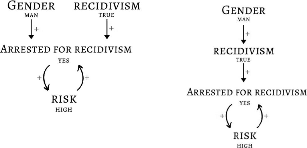
Figure 1: Causal models of biased (left) and unbiased (right) risk assessment
The idea is to be able to evaluate the effect of survivorship bias mitigation on the performance of the prediction tool over a period of time. In order to do this, we assume that one learning cycle represents one year. Every year new individuals will get arrested and therefore become part of the dataset. However, this is influenced by the composition of the people that offend, further referred to as the reality, and possible bias. Subsequently, the composition of the new individuals will be different in the fair situation compared to the unfair situation. It is assumed that in the unfair situation, an equal amount of men and women recidivate. Therefore, the dataset of the unfair reality will consist of an equal amount of male and female individuals. Moreover, half of the population recidivate and half offend for the first time. In the unfair reality, there exists a bias towards men, thus men have a larger probability of getting arrested compared to women. Consequently, it will seem like men recidivate more often than women. In the fair situation, the assumption that men recidivate more is true. The percentage of men with a high risk label is larger compared to the percentage of women with a high risk label. In this case, the dataset still consists of an equal amount of men and women, but 70% of the male population and 50% of the female population have a high risk label. However, men and women have the same chance of getting arrested.
| Noise | Options | Percentage |
| Age | 0-100 | Gaussian distribution |
| Educational level | ‘A’, ‘B’, ‘C’, ‘D’ | 25% each |
| Crime rate | 1, 2, 3, 4 | 25% each |
| Criminal history | ‘Yes’ (1) or ‘No’ (0) | 50% each |
Table 1: Noise attributes with their distribution
In both realities the chance that a criminal will get arrested is two third and the probability of being a men or women is 50%. Moreover getting arrested given a high predicted risk score increases the probability of getting arrested to 70% compared to 50% for individuals with a low predicted risk. Each learning cycle, a new dataset of 5,000 individuals is evaluated and based on their gender and predicted risk they are added to the dataset. The conditional probabilities determine how many individuals of each group are added to the subset of the reality.
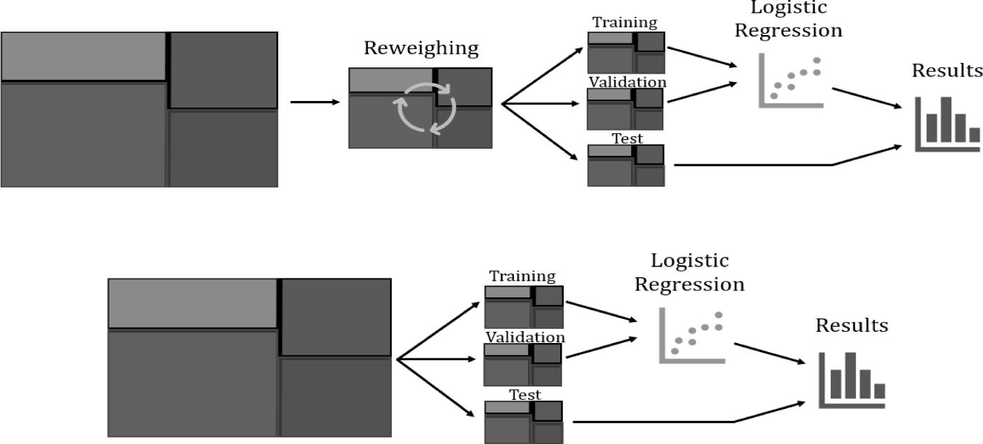
Figure 2: One learning cycle, with debiasing (top) and without (bottom)
4.
Results ^
When 70% males and 50% females recidivate, all men are classified as high risk and about 30% of women as low risk. After reweighing, all individuals are classified as high risk. The accuracy of the first round of each situation varies around 62%. This is logical, since almost all individuals are classified as high risk and about 62% of the population has a high risk label in reality. Most interesting is the fair situation with debiasing. We expected a significant decrease of the accuracy since the prediction of high risk will be decreased by debiasing while there was no bias in reality. However, both with and without debiasing, the accuracy varies barely (–1.2% and –1.5%). In the unfair situation the accuracy decreased 7.3 (debiasing) and 7.7% (no debiasing).
When 40% of males and 30% of females recidivate, almost all individuals have a low predicted risk. Without debiasing the few people that have a high risk label are male. With debiasing, also a few women receive a high risk score. The accuracy with and without debiasing decreases about 8%. In the fair situation, with debiasing, still almost all individuals are labelled as low risk. However, an increasing amount of women and men are classified as high risk individuals. The accuracy decreases with 12.4%. Without debiasing, the amount of men classified as high risk increases fast; from 5 to 2326 in 5 rounds. Almost no women receive a high risk label. The accuracy decreases with 8.4%. Thus, in the 40/30 situation, the accuracy of the fair situation with debiasing meets our expectation.
When 10% of males and 3% of females recidivate, almost all individuals are labelled as low risk. Accuracy decreases significantly over time; 23% in the unfair and 26% in the fair situation. This can be explained by the addition of high risk individuals each round.
5.
Conclusions and Discussion ^
A lot of information can be found on detecting bias, notions of fairness and bias mitigation; far less on exploring the causes and effects of bias. The design choices of our simulation tool cannot yet be supported by research or real cases. Subsequently, the correctness of the design choices are open for discussion.
This paper explores effects of data settings rather than the effect of survivorship. The percentage of high risk labelled individuals of the total dataset has a clear effect on the predictions of the recidivism prediction tool. When initially more than half of the population recidivate, the prediction tool will classify all individuals as high risk. On the other hand, when a small percentage has a high risk label, each individual will be labelled as a low risk. The hypothesized effect, where the accuracy decreases specifically in the fair situation with debiasing, was best seen in the 40/30 situation. This suggests that the composition of the start dataset has an influence on the possibility to observe the effect of bias mitigation on performance.
In order to be able to draw conclusions about the effect of survivorship bias mitigation itself, more research has to be done with a proper, realistic dataset. This research is just a first step.
6.
References ^
- Rachel K. E. Bellamy et al. “AI Fairness 360: An Extensible Toolkit for Detecting, Understanding, and Mitigating Unwanted Algorithmic Bias”. In: CoRRabs/1810.01943 (2018). arXiv: 1810.01943. url: http://arxiv.org/abs/1810.01943.
- Julia Dressel & Hany Farid. “The accuracy, fairness, and limits of predicting recidivism”. In: Science Advances (2017). issn: 2375-2548. url: https://doi.org/10.1126/sciadv.aao5580.
- Gonzalo Ferreiro Volpi. “Survivorship bias in Data Science and Machine Learning”. In: Towards Data Science (2019). url: https://towardsdatascience.com/survivorship-bias-in-data-science-and-machine-learning-4581419b3bca.
- 1 Gonzalo Ferreiro Volpi. “Survivorship bias in Data Science and Machine Learning”. In: Towards Data Science (2019). url: https://towardsdatascience.com/survivorship-bias-in-data-science-and-machine- learning-4581419b3bca.
- 2 Rachel K. E. Bellamy et al. “AI Fairness 360: An Extensible Toolkit for Detecting, Understanding, and Mitigating Unwanted Algorithmic Bias”. In: CoRRabs/1810.01943 (2018). arXiv: 1810.01943. url: http://arxiv.org/abs/1810.01943.
- 3 Julia Dressel & Hany Farid. “The accuracy, fairness, and limits of predicting recidivism”. In: Science Advances (2017). issn: 2375-2548. url: https://doi.org/10.1126/sciadv.aao5580.
- 4 Julia Dressel & Hany Farid. “The accuracy, fairness, and limits of predicting recidivism”. In: Science Advances (2017). issn: 2375-2548. url: https://doi.org/10.1126/sciadv.aao5580.


